Machine Learning #2: Regression Models
Linear Regression (OLS)
The terms Linear Regression and Ordinary Least Squares can be used interchangeably as they both fit data by minimizing the sum of square differences between the observed and predicted values.
The input, output, & action spaces are defined $X: \mathbb R^P$, $y: \mathbb R$, $A: \mathbb R$
Assuming $\beta_0$ is the intercept and $x_0 = 1$:
$\forall$ means ‘for all’, then to find the best $\beta$:
\[\hat \beta = argmin_\beta \hat R(\beta ^T x)\] \[= argmin_\beta \frac1N \sum_{i=1}^N (y^{(i)} - \beta ^ T x^{(i)})\]Then, the Empirical Risk Minimizer is:
\[\hat f = argmin_{f \in \mathscr F} \hat R(f)\] \[\hat f(x) = \hat \beta ^T x = \sum_{i=0}^P \hat \beta _i x_i\]These equations are all the same as the definitions, except that the predicted value is represented by $\beta ^ T x^{(i)}$ and the actual value by $y^{(i)}$.
Example: Predicting life satisfaction from GDP & gender
$\beta _0 + \beta _1GDP + \beta _2NumChildren$
Then $x_0 = 1$, $x_1 = GDP$, $x_2 = NumChildren$
Code
The following is Python code to implement the sklearn Linear Regression algorithm.
As this is a continuous function, the performance can be measured using mean squared error.
from sklearn.linear_model import LinearRegression
from sklearn.metrics import mean_squared_error
from sklearn.model_selection import train_test_split
The data is split into training and testing subsets then the model is defined and fit to the training data.
train, test = train_test_split(data, test_size = 0.2, random_state = 1)

model = LinearRegression()
model.fit(train[['inputs']], train['y'])
A linear regression model has intercept and coefficient attributes that can be found using .intercept_ and .coef_.
print('Intercept: {}, Coefficient: {}'.format(model.intercept_, model.coef_))
A column of predicted values is added to the test dataset
test['y_pred'] = model.predict(test[['inputs']])
We can get the MSE of the predictions.
print(mean_squared_error(test['y'], test['y_pred']))
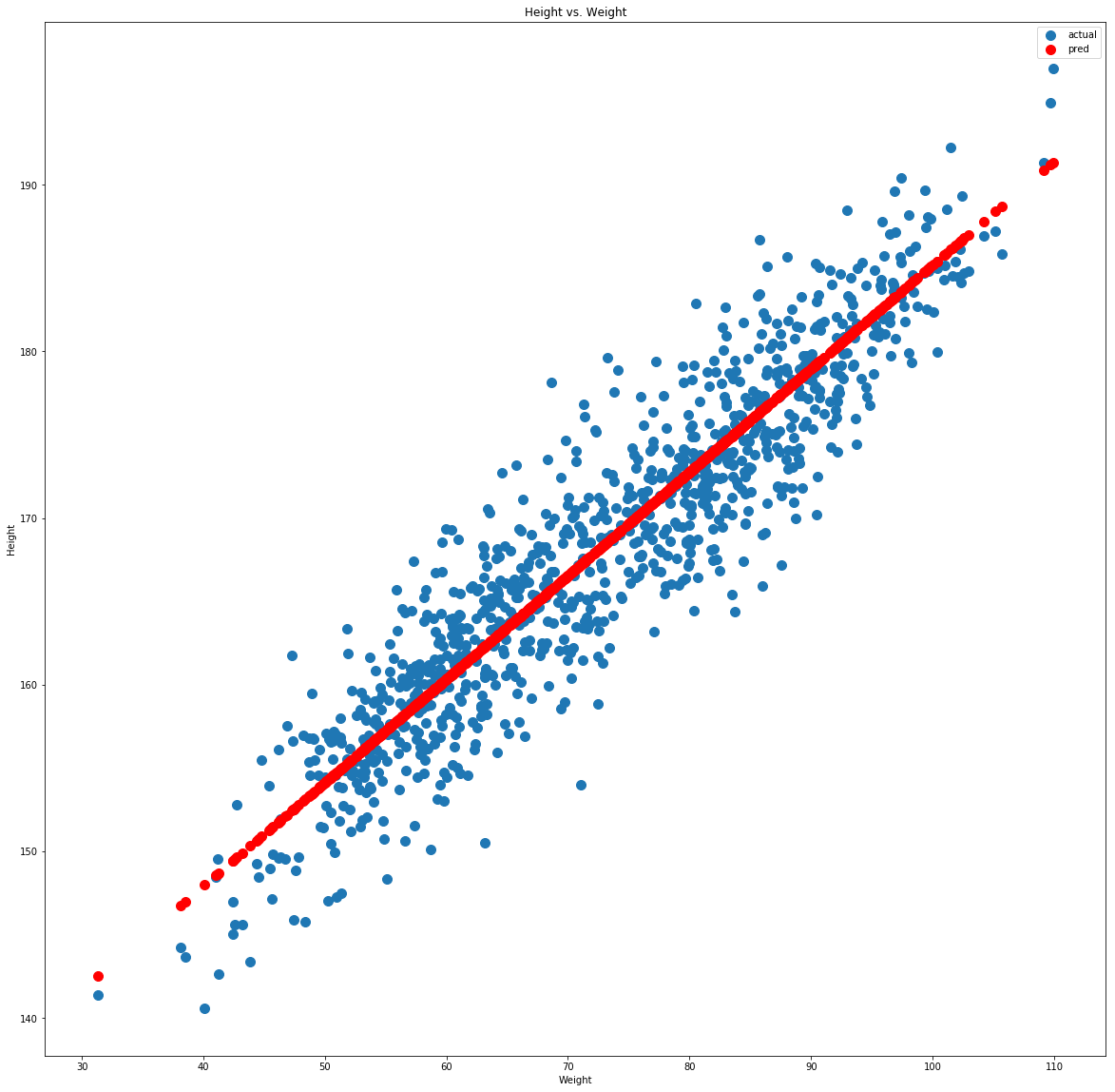
We can plot the actual values against the predicted values to get a visual idea of performance.
import matplotlib.pyplot as plt

fig, ax = plt.subplots(figsize=(20,20))
ax.scatter(test['inputs'], test['y'], s=100, label='actual')
ax.scatter(test['inputs'], test['y_pred'], s=100, c='r', label='prediction')
ax.legend()
Logistic Regression
Despite its name, logistic regression is not regression, it is actually used for binary classification. This is the same as giving the probability that y=1 for each case of x:
\[\hat f(x) = P(y=1|X=x)\]Spaces
$X = \mathbb R^P$
$y = {0,1}$ (Only 0 or 1)
$A = (0,1)$ (Any no. from 0-1)
Sigmoid Function
The sigmoid function is used as a means of normalization for logistic regression (and neural networks) as it maps numbers in $\mathbb R$ to the open interval (0,1). As x gets larger sigmoid(x) tends to 1, as x gets smaller it tends to 0 but will never be exactly either 0 or 1.
\[\sigma (x) = \frac1{1+ e^{-x}}\]We assume $x_0=1$ so $\beta _0$ is the intercept term. P is the number of predictors (+1 is for the $\beta _0$ term). Then the hypothesis space is defined:
\[\mathscr F = \{sigmoid(\beta ^T x) | \beta \in \mathbb R ^ {P+1}\}\]Loss Function
The loss function for logistic regression is the log loss:
\[L(y, \hat y) = -(ylog(\hat y) + (1-y)log(1- \hat y))\]Log loss can be derived from maximum likelihood estimation.
Likelihood Estimation
If $\bar y$ is a vector of all outcomes, $X$ is a matrix of all inputs and assuming conditional independence: \(\alpha (\beta) = P(\bar y | X; \beta) = \prod ^N_{i=1} P(y^{(i)} | x^{(i)} ; \beta)\)
This is the probability of $y$ given $X$ parameterized by $\beta$.
In the case where $y \in {0,1}$
\[\alpha (\beta) = \prod ^N_{i=1}\sigma (\beta ^T x^{(i)})^{y^{(i)}}(1-\sigma (\beta ^T x^{(i)})^{1-y^{(i)}}) = \prod ^N_{i=1}\sigma (\hat y^{(i)})^{y^{(i)}}(1-\hat y^{(i)})^{1-y^{(i)}}\]If $y^{(i)}$ is 1 the right term will cancel, if $y^{(i)}$ is 0 the left term will cancel. In either case the other term will be maximized. This means that the $\beta$ that maximizes the log likelihood is the same that will mazimize the likelihood.
Empirical Risk Minimizer
The target function to be minimized is the empirical risk of the prediction function with respect to $\beta$.
\[J(\beta) = \hat R(f) = \hat R(sigmoid(\beta ^Tx)) = \hat R(\sigma (\beta ^ TX))\]The $\beta$ value that produces the lowest empirical risk is denoted by $\hat \beta$.
The prediction function is then
\[\hat y = \hat f(x) = sigmoid(\beta ^ Tx)\]This tends to 1 as $\beta ^ Tx$ gets large and tends to 0 as $\beta ^ Tx$ gets largely negative.
Code
The following is Python code to implement the sklearn Logistic Regression algorithm.
As a classification algorithm, performance of logistic regression can be measured by accuracy or log loss.
from sklearn.linear_model import LogisticRegression
from sklearn.metrics import accuracy_score, log_loss
from sklearn.model_selection import train_test_split
Perform the train-test split then define and fit model as usual.
train, test = train_test_split(data, test_size = 0.2, random_state = 1)

model = LogisticRegression()
model.fit(train[['inputs']], train['y'])
Create new columns with the class prediction and probability of possitive classification respectively then output accuracy, log loss, intercept, & coefficients.
test['y_pred'] = model.predict(test[['inputs']])
test['y_prob'] = model.predict_proba(test[['inputs']])[:,1]

loss = log_loss(test['y'], test['y_pred'])
accuracy = accuracy_score(test['y'], test['y_pred'])

print('Accuracy: {}%\nLoss: {}\nIntercept: {}\nCoefficient: {}'.format(accuracy * 100, loss, model.intercept_, model.coef_))
Accuracy: 85.11488511488511%
Loss: 5.141190065803713
Intercept: [-43.89196847]
Coefficient: [[0.26042762]]
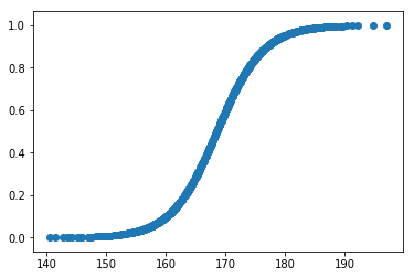
The prediction function is then $f(x) = sigmoid(-43.89 + 0.26*Height)$
The prediction function can be visualised with a scatter plot
import matplotlib.pyplot as plt

fig, ax = plt.subplots()
ax.scatter(test['y'], test['y_prob'])
Polynomial Regression
If we have a non-linear relationship between x and y then our model must take the form \(\hat y = \hat \beta _0 + \hat \beta _1 x + \hat \beta _2 x^2 + \hat \beta _3 x^3 + ...\)
Taylor Series
The taylor series is an inifite sum evaluated at polynomial steps, it can be used to expand a continuous function. For example, expanded at 0:
\[f(x) = f(0) + f'(0)x + \frac12f''(0)x^2 + \frac16f'''(0)x^3 + ...\] \[f(x) = \sum _{i=0}^{\infty}\frac1{i!} f^{(i)}(0)x^i\] \[f(x) = \sum _{i=0}^{\infty} \beta _i x^i\]We can solve the last equation using polynomial regression where $\beta = \frac1{i!} f^{(i)}(0)$.
Limitations
Polynomial regression usually behaves well on the data range in question, for x values outside the bounds of the training data it can be unpredictable. When predicting, you should be sure that the x you are predicting for is within the range of the training data.
Constrained Regression
Linear regression doesn’t work well when there is noise or outliers. Constrained regression minimizes the effect of these outliers using norms.
$L^2$ Norm
A measure of the size of a vector, the $L^2$ norm is the same as the distance measure used in pythagoras ($\sqrt{a^2 + b^2}$).
\[||\beta||_2 = (\beta _1^2 + \beta _2^2 + ... + \beta _P^2)^{\frac12}\]$L^q$ Norm
The general form of $L^2$ norm where the power and root is $q$.
\[||\beta||_q = (\beta _1^q + \beta _2^q + ... + \beta _P^q)^{\frac1q}\]Ridge Regression
Ridge regression is Ordinary Least Squares with an $L^2$ norm penalty. The spaces are defined by the following (same as OLS):
$X: \mathbb R^P$
$y: \mathbb R$
$A: \mathbb R$
$\mathscr F:{b + \beta ^Tx |b \in \mathbb R, \beta \in \mathbb R^ P}$
We penalise the norm of $\beta$ in order to tend to solutions that are less sensitive to changes in the input.
\[J(\beta , b) = \frac1N \sum _{i=1}^N (y^{(i)} - b + \beta ^Tx^{(i)})^2 + \lambda ||\beta||_2^2\]It is normal to standardise predictors before applying ridge regression.
\[\hat \beta, \hat b = argmin_{\beta, b} J(\beta, b)\]Then the prediction function is the same as linear regression \(\hat f = \hat b + \hat \beta ^Tx\)
When lambda=0 the function is OLS, when lambda=1 the function is constant without any coefficients. Generally, for an increasing $\lambda$ the approximation error will increase while estimation error decreases. The generalization error will increase. This is generally true for increased complexity compared to model performance.
Code
Ridge regression can be implemented with the sklearn ridge module. The standard scaler is also used to standandardise the dataset before training.
from sklearn.linear_model import Ridge
from sklearn.preprocessing import StandardScaler
from sklearn.model_selection import train_test_split

train, test = train_test_split(data, test_size = 0.2, random_state = 1)
A scaler must be defined, before .fit_transform is applied to the training set and .transform to the test set.
scaler = StandardScaler()
train_scaled = scaler.fit_transform(train['inputs'])
test_scaled = scaler.transform(test['inputs'])
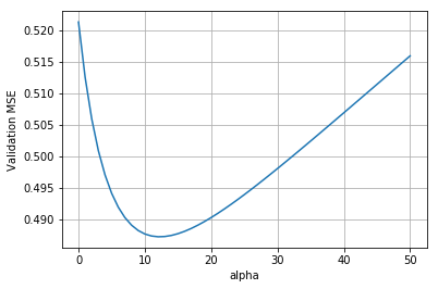
Here, ridge regression is applied for varying $\lambda$ / alpha values. The results for each alpha are stored in a dictionary, the coefficients for each model are also stored.
results = {}
reg_paths = {}

for alpha in np.linspace(0,50,51):
    model = Ridge(alpha=alpha)
    model.fit(train_scaled, train['y'])

    # Tracking coefficients
    coefs = dict(zip('inputs', model.coef_))
    reg_paths[alpha] = coefs

    # Tracking validation error
    test_scaled['y_pred'] = model.predict(test_scaled)
    test_mse = mean_squared_error(test_scaled['y'], test_scaled['y_pred'])

    results[alpha] = test_mse

df_coefs = pd.DataFrame(reg_paths).T
We can then plot the validation mean squared error as a function of alpha
import matplotlib.pyplot as plt

fix, ax = plt.subplots()
ax.plot(results.keys(), results.values())
ax.set_xlabel('alpha')
ax.set_ylabel('Validation MSE')
ax.grid()
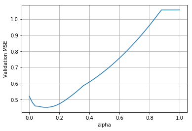
Lasso Regression
This is the same as ridge regressions except it penalises on $||\beta||_1$ instead of $||\beta||_2^2$.
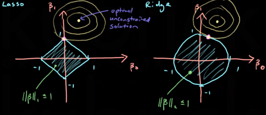
\[||\beta||_1 = (\beta _1 + \beta _2 + ... + \beta _P)\]The Lasso will return sparse solutions with many 0’s in the $\beta$ vector. The ridge does not do this. This is because the contours of the objective function is more likely to intersect the lasso penalisation area where one of the $\beta$ values is 0.
Lasso regression can be implemented with the sklearn lasso module. It is applied in exactly the same way as the ridge. The loss v alpha plot is shown below.