Machine Learning #3: Classification Models

7 minute read

Support Vector Classification

SVC is a classification algorithm where the prediction function is a score function the output of which is a real number that represents the level of confidence in a positive class.
$X: \mathbb R^P$
$y: {-1,1}$
$A: \mathbb R$
$\mathscr F: {b+\beta ^T x |b \in \mathbb R, \beta \in \mathbb R^P}$

Margin is a measure of correct classifications. A positive margin means we have classified correctly and inverse for a negative margin. A highly positive margin is generally a good marker for the classifier.
margin = $y * \hat f(x)$ = actual * predicted score

Objective Function

The SVC objective function is just the average hinge loss of the predictions with a regularisation term $\lambda

\beta

^2_2$ applied to reduce complexity.

\[J(\beta, b) = \lambda ||\beta ||^2_2 + \frac1N \sum _{i=1}^N max(0, 1 - y^{(i)}(b + \beta ^T x^{(i)}))\] \[(\hat \beta, \hat b) = argmin_{\beta, b}J(\beta, b)\]

Prediction function: $\hat f = \hat b + \hat \beta ^Tx$

The SVC gives us a hyperplane that attempts to separate the positive and negative classes. Set $\hat f(x) = 0$ to see the decision boundary.

Code

Support Vector Classification can be implemented using the sklearn linear SVC module

from sklearn.svm import LinearSVC

model = LinearSVC()
model.fit(train['inputs'], train['y'])

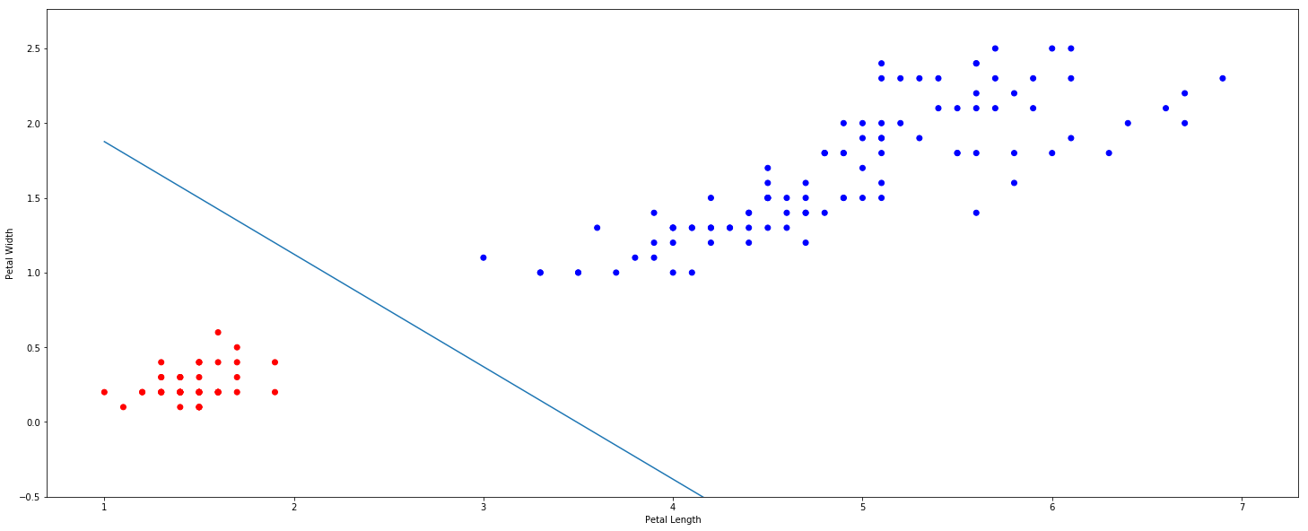
We can plot the decision boundary created by the classifier, this example uses the Iris dataset.

import matplotlib.pyplot as plt

fig, ax = plt.subplots(figsize = (25,10))
ax.scatter(df['petal length (cm)'], df['petal width (cm)'], 
           c=df['IsSetosa'].map({1:'red', 0:'blue'}))
ax.set_xlabel('Petal Length')
ax.set_ylabel('Petal Width')

x = np.linspace(1,7,10)
y = (-0.61*x + 2.13)/0.81

ax.plot(x,y)
ax.set_ylim(-0.5)

K-Nearest Neighbours

KNN is a prediction method that classifies a new point based on the class and euclidean distance ($L^2$ norm) of its K nearest neighbours. K is a hyperparameter and is set in advance, KNN is also non-parametric meaning we do not know the number of parameters before fitting. The set of K nearest points to x is denoted by $N_K(x)$.

The prediction for regression is the average value of the K-nearest neighbours:

\[\hat y = \hat f(x) = \frac1K \sum_{i:x^{(i)} \in N_K(x)} y^{(i)}\]

For classification we find the probability that x is in some class c. The 1 denotes an indicator function (1 when y=c, 0 otherwise).

\[\hat y_c = P(y=x|X=x) = \frac1K \sum_{i:x^{(i)} \in N_K(x)} 1(y^{(i)}=c)\]

Choosing K

The choice of K affects the complexity of the model. A large K will be very robust but not sensitive (underfitting), whereas a small K will be highly sensitive to the training data (overfitting).

Example: If there is a single blue point in a sea of yellows and a new point next to it must be classified. K=1 will classify it as blue, K>1 will classify it as yellow which is more realistic.

Limitations

KNN must store all the training data for the model which can be a problem with a large dataset.
KNN suffers from ‘the curse of dimensionality’ meaning it fails to perform well with many predictors.
KNN is sensitive to the scale of the data

Code

K-Nearest Neighbours can be implemented with the sklearn K Neighbors Classifier.

from sklearn import neighbors
from sklearn.model_selection import train_test_split
from sklearn.metrics import accuracy_score

Split data, define & fit KNN model, make predictions then print accuracy

train, test = train_test_split(data, test_size = 0.2, random_state = 1)

clf = neighbors.KNeighborsClassifier(k)
clf.fit(train[['inputs']], train['y'])
test['y_pred'] = clf.predict(test[['inputs']])

print('Accuracy: {}%'.format(round(accuracy_score(test['y'], test['y_pred']), 2) * 100))

Classification and Regression Trees (CART)

Decision trees classify data points into buckets, represented by leaf nodes. The starting node is the root node and nodes inbetween are internal nodes. Between each node level some equality expression is applied.

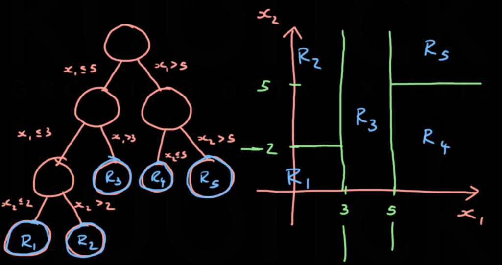
We only consider binary splits of the form $x_j \leq c; x_j \geq c$. With CART each region is associated with a single constant prediction, two different points will be treated the same as long as they’re in the same region.

The prediction function for a tree is given as

\[\hat y = \hat f(x) = \sum _{m=1}^M c_m 1(x \in R_m)\]

This predicts $c_m$ if $x$ falls in the region $R_m$, $M$ is the number of regions.

Characterizing splits

To define the split of a set of variables $(x_1 … x_P)$ we need:

A splitting variable $j \in {1,2…P}$ which describes the variable/dimension to split by
A split point $s \in \mathbb R$ which decribes where to split the variable $j$

Recursive Binary Splitting Algorithm

This is a greedy algorithm for growing classification and regression trees. Assuming a squared error loss, the prediction is just the average $y^{(i)}$ for each region $R$.

\[\hat c_m = \frac1{N_m} \sum_{\{i:x^{(i)} \in R_m\}} y^{(i)}\]

The left and right regions for a given $j$ and $s$ are mathematically defined by:

\[R_L(j,s)=\{x|x_j \leq s\}\] \[R_R(j,s)=\{x|x_j \geq s\}\]

The prediction for each region is then defined by:

\[\hat c_L(j,s) = avg(y^{(i)}|x^{(i)} \in R_L(j,s))\] \[\hat c_R(j,s) = avg(y^{(i)}|x^{(i)} \in R_R(j,s))\]

The regression loss function is the combined sum of squared errors for each region

\[L(j,s) = \sum _{\{i:x^{(i)} \in R_L(j,s)\}} (y^{(i)} - \hat c_L(j,s))^2 + \sum _{\{i:x^{(i)} \in R_R(j,s)\}} (y^{(i)} - \hat c_R(j,s))^2\]

Our aim is the find $j$ and $s$ such that $L(j,s)$ is minimized, this will correspond to the best greedy split. The algorithm should then be applied recursively to each new region to split into smaller regions.

Given N data points & P dimensions, for each dimension there are at most N-1 possible splits. Therefore, using brute force we need to try at most P(N-1) splits.

Variable Importance

The importance of variable $j$ in tree $T$ is the sum of improvements from splitting on $j$.

The improvement of $j$ on $T$ is defined as

\[I_j(T) = \sum^J_{t=1}\tau_t 1(v(t) = j)\]

Where $\tau_t$ is the improvement at node $t$ and the indicator function $1$ outputs 1 when the split is on variable $j$.

Entropy

Entropy is a measure of disorder and can be used to measure the performance of a decision tree via the information gain metric. At each split the entropy of the data at the node should decrease as the data becomes more ordered.

Information Gain:

\[-\sum_{j=1}^Jp_jlog_2p_j\]

For $J$ labels, each with a ratio of $p$ in the set.

Gini Impurity

Closely related to information gain, the gini impurity is also called the logical entropy. The gini impurity is a measure of the likelihood of an incorrect classification based purely on the existing data. This can be used interchangeably with information gain althought gini doesn’t require $log$ so is faster to compute.

Gini Impurity:

\[1-\sum_{j=1}^Jp_j^2\]

Preventing Overfitting

If we keep applying the splitting algorithm it may make a region for each individual point. We can control complexity by

Setting a minimum number of points for each region / leaf node
Limit the depth of the tree
Stop splitting when the reduction in loss is under some threshold
Don’t split a node if the number of points is too small

Decision trees generally suffer from high variance, this can be remedied using random forests

Bagged Trees

Bagged trees is just applying bagging to a tree prediction function.

Sample B bootstrapped datasets
Train B trees
Take average

As bagging reduces variance it allows for deeper, more complex trees to be used.

Hyperparameters

All hyperparameters for trees
Number of trees, B (more trees cannot negatively affect performance, but will be slower)

Code

The code to implement a decision tree is similar to that of logistic regression. This example uses the scikit-learn Decision Tree Classifier.

from sklearn.tree import DecisionTreeClassifier
from sklearn.metrics import accuracy_score
from sklearn.model_selection import train_test_split

Split then define and fit model as usual, then make predictions and print out the accuracy

train, test = train_test_split(data, test_size = 0.2, random_state = 1)

model = DecisionTreeClassifier()
model.fit(train[['inputs']], train['y'])

test['y_pred'] = model.predict(test[['inputs']])
test['y_prob'] = model.predict_proba(test[['inputs']])[:,1]

print('Accuracy: {}%'.format(round(accuracy_score(test['y'], test['y_pred']), 2) * 100))

A visual representation of the tree can be exported using the export_graphviz module.

Random Forests

Random forests is like an extension of bagged trees. Only a random subset of predictors (j) can be chosen at each splitting step of a tree. This adds randomness to the tree growth to make the trees less correlated.

Hyperparameters

No. of trees
No. of candidate predictors at splitting step
All hyperparameters for trees

Variable Importance

The variable importance in a bagged tree or random forest is defined as the average improvement over all trees when using $j$ as the split variable.

\[I_j(F) = \frac 1B \sum^B_{i=1} I_j(T_i)\]

K-Means Clustering

K-Means is a clustering algorithm, and an example of non-supervised learning. It partitions data into K clusters.

Standardize data
Initialize cluster centres ($\mu$)
Repeat until convergence:
- Assign each point to the cluster with closest centre
- Update cluster centres

The output of K-means can be used as an input to a supervised algorithm.

Another clustering algorithm is DBSCAN.

Naive Bayes Classification

Bayes Theorem:

\[P(A|B) = \frac{P(B|A)P(A)}{P(B)}\]

With naive bayes we assume that the data comes from a model where $y$ influences all $x$’s and each $x$ is independent from eachother (hence naive).

We know in this case: $P(x_1) = P(x_1|y)P(y)$

Therefore $P(y, x_1, x_2) = P(x_1|y)P(x_2|y)P(y)$

Example:
Classifying spam email where y=Spam, $x_1$=All Caps, $x_2$=Contains ‘FREE’
Suppose we know $P(y)$, $P(x_1)$, $P(x_2)$ then, by Bayes:

$P(y|x_1,x_2) = \frac{P(x_1, x_2|y)P(y)}{P(x_1, x_2)}$

Naive Bayes is a very good classifier and can outperform most others if you can guarantee independent predictors (not easy).