Machine Learning #4: Model Optimization
Feature Engineering
Feature engineering requires using domain knowledge to make better predicting features from the input data. For example, given GDP and population a new feature could be GDP per capita or the log of GDP per capita and these may perform better as a predictor on a model.
One-Hot Encoding
One-hot encoding aka ‘dummy variables’ is a method of converting strings to binary so that an algorithm can understand and compress the information. For each string value in a category a new binary truth column is created.
Example: ‘Dog’ -> 1 0 0, ‘Cat’ -> 0 1 0, ‘Rat’ -> 0 0 1
Feature Maps
A feature map $\Phi$ is a function mapping a raw vector input $x$ to a new vector that is used in a model.
\[\Phi: \mathbb R^P \to \mathbb R^q\]Example: Mapping weight & height to BMI
Feature Selection
Selecting a sub-set of features to use in the prediction model. This can be done manually or automatically by a feature selecting algorithm.
The coefficient associated with a feature is not a good predictor of importance as the features are often on different scales. If we standardise features (minus column mean, divide by stdev) and then perform regression then the coefficients can be compared for relative feature importance.
Example: $\hat y = 10x_1 + 0.2x_2 + 5$
If $x_1$ and $x_2$ are standardised then we can say that $x_1$ is a more important feature as $\beta _1 = 10$
Best Subset Selection
For a set of features ${x_1, x_2, x_3, … ,x_P}$ best subset selection is the subset of features such that the generalization error is minimized. For $P$ features we must test $2^P$ models which is very computationally expensive, therefore it only works for a small $P$.
Forward Step-Wise Selection
Given $p$ predictors;
- Start with constant model $\hat f_0 = \beta _0$
- For $i$ from $1$ to $p$:
- Find the best predictor $x_*$
- Add $x_*$ to predictors used in $\hat f_{i-1}$
- Result is a sequence of models, Eg;
- $\hat f_0 = \hat \beta _0^0$
- $\hat f_1 = \hat \beta _0^1 + \hat \beta _3^1x_3$
- $\hat f_2 = \hat \beta _0^2 + \hat \beta _3^2x_3 + \hat \beta _5^2x_5$
- $\hat f_3 = \hat \beta _0^3 + \hat \beta _3^3x_3 + \hat \beta _5^3x_5 + \hat \beta _1^3x_1$
- Evaluate each model from the sequence on the test set and choose the best
The $\hat \beta$ values are different for each iteration. Each iteration uses all the features from the previous iteration. This is always done only on the training data.
Regularization
It is common for test error to decrease with some added complexity but to then increase with too much added complexity as the models tends to start overfitting. Regularization is used to reduce model complexity, mostly to reduce overfitting.
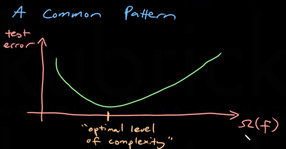
Complexity Measure
The complexity measure $\Omega$ of $f$ is a functional that measures complexity.
\[\Omega (f): \mathscr F \to [0,\infty]\]Ivanov Regularization
AKA constrained regularization.
\[\hat f = argmin_{f \in \mathscr F} \hat R(f)\]Such that $\Omega(\hat f) \leq c$
Tikhonov Regularization
AKA penalised regularization, a $\lambda$ term is used as a penality for complexity.
\[\hat f = argmin_{f \in \mathscr F} \hat R(f) + \lambda \Omega (f)\]Where $\lambda \geq 0$
In many cases, when c and $\lambda$ are equivalent: Ivanhov and Tikhonov regularization gives the same prediction function.
Model Averaging
Model averaging can reduce overfitting without changing the expectation.
Given $B$ independent training sets of equal size we can train $B$ independent prediction functions $(\hat f_1, … \hat f_B)$.
The model average over $B$ is defined \(\hat f_{avg} = \frac 1B \sum ^B_{i=1} \hat f_i\)
\(E[\hat f(x_0)] = \frac 1B E[\sum ^B_{i=1} \hat f_i(x_0)]\) \(= \frac 1B \sum ^B_{i=1} E[\hat f_1(x_0)]\) \(= E[\hat f_1(x_0)]\)
This shows that model averaging does not change the expected prediction.
\(var(\hat f_{avg}(x_0)) = var(\frac 1B \sum ^B_{i=1} \hat f_i(x_0))\) \(= \frac 1B var(\hat f_1(x_0))\)
This shows that model averaging can reduce the error due to variance.
However, in real life we do not have $B$ independent datasets.
Bagging
Bagging, also known as bootstrap aggregation is used when we want to decrease the model variance while retaining a level of bias. It is a special case of model averaging. First we must bootstrap the dataset, taking the average of the bootstrapped datasets is bagging.
Bootstrapping
Bootstrapping is a term that can be applied to any process involving random sampling with replacement (each value returns to dataset after it’s sampled).
Given a dataset of size N:
- Repeat for i from 1:B
- $D_i$ = randomly drawn set of points (with replacement)
- Result is B boostrapped datasets ($D_1$, $D_2$ … $D_B$)
Bootstrap Aggregation
Train B prediction functions on B bootstrapped datasets: $\hat f_1, \hat f_2 … \hat f_B$.
Take the average to reduce the variance
\[\hat f_{avg} = \frac 1B \sum^B_{i=1} \hat f_i\]The theoretical variance is $\frac 1B var(\hat f_1(x_0))$. In practice the variance will be higher since the training sets are never totally independent. Bagging still works well when the prediction function suffers from high variance.