Machine Learning #5: Model Evaluation
Model Diagnostics
Improving a model with high errors on both the training and test sets:
- Try a more flexible or complex model
- Construct new features
Improving a model with low training error but high test error (overfitting):
- Feature selection
- Bootstrap aggregation
- Try simpler model
- Regularization
- Gather more data
Learning Curves
Learning curves plot error against training set size. They’re used to diagnose underfitting or overfitting.
An underfit model has a high training error and a high test error
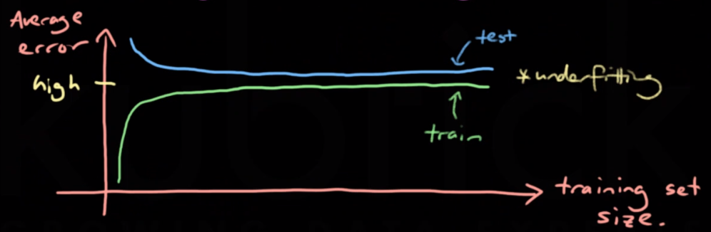
An overfit model has a low training error but a high test error
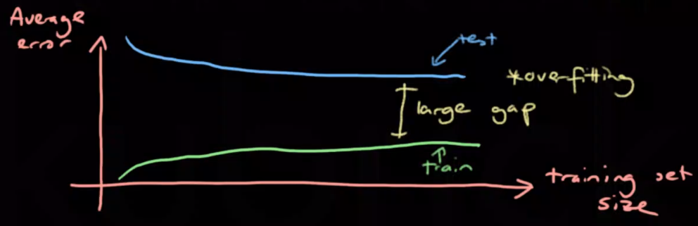
A perfect model with have low training and testing error.
Evaluating Regression Models
Evaluating regression models usually involves a form of loss function.
| Error | Equation | Description |
|---|---|---|
| Mean absolute error | $\frac 1N \sum _{i=1}^N |y^{(i)} - \hat y^{(i)}|$ | Pure magnitude of error |
| Mean Squared | $\frac 1N \sum _{i=1}^N (y^{(i)} - \hat y^{(i)})^2$ | Measure of error magnitude with extra emphasis on large errors |
| Root mean squared | $\frac 1N \sum _{i=1}^N \sqrt{(y^{(i)} - \hat y^{(i)})^2}$ | Measure of euclidian distance of error, extra emphasis on large errors |
| $R^2$ | $1 - \frac{RSS}{TSS}$ | How well the model performs compared to a constant model |
| RSS/TSS | $RSS = \sum _{i=1}^N (y^{(i)} - \hat y^{(i)})^2$, $TSS = \sum _{i=1}^N (y^{(i)} - avg(\hat y^{(i)}))^2$ | Risidual sum of squares and Total sum of squares |
| MAPE | $\frac{100}{N} \sum ^N_{i=1}|\frac{x_i - \hat x_i}{x_i}|$ | Mean absolute percentage error |
| SMAPE | $\frac{100}{N} \sum ^N_{i=1}|\frac{2(x_i - \hat x_i)}{x_i + \hat x_i}|$ | Symmetric mean absolute percentage error |
Evaluating Classifiers
Classification accuracy gives a measure of performance but does not reveal the types of errors that are being made.
Confusion Matrix
Shows where misclassifications are false positives or false negatives.
| Predicted | Actual 0 | Actual 1 |
|---|---|---|
| 0 | TN | FN |
| 1 | FP | TP |
Depending on the application it may be more important to put emphasis on particular types of error. For example false negatives definitely want to be avoided when diagnosing a serious illness.
Given a model predicting the probability of an observation being positive. We can choose a cutoff c such that we predict positive if $\hat f(x) \geq c$ and negative otherwise.
A higher c value will increase the TRUE POSITIVE rate but FALSE POSITIVE will also increase.
A low c value will increase TRUE NEGATIVE but FALSE NEGATIVE will also increase.
True Positive Rate (TPR)
\[TPR = \frac{TP}{P} = \frac{TP}{TP + FN}\]If c=0, TPR = 1 & TNR = 0
True Negative Rate (TNR)
\[TNR = \frac{TN}{N} = \frac{TN}{TN + FP}\]If c=1, TNR = 1 & TPR = 0
ROC Curve
ROC (Reciever Operating Characteristic) curves show how well a classifier separates positive and negative classes and the trade-off between the TPR and the TNR as the cut-off c is varied. The x axis is $1-TNR$ and the y-axis is $TPR$, a curve that hugs the upper left corner represents a better classifier.
The area under the curve is called the ROC AUC, it tells us how well ranked our predictions are. An ROC AUC of 1 means we have a perfect classifier meaning some cutoff c exists that will perfectly distinguish positive and negative classes. ROC AUC of 0.5 is equivalent to a random guess.
Code
The ROC curve and ROC AUC can be found using the sklearn ROC curve and ROC AUC score modules respectively.
from sklearn.metrics import roc_curve, roc_auc_score
Assuming a fitted logistic regression model
y_prob = model.predict_proba(test[['inputs']])[:,1]

fpr, tpr, threshold = roc_curve(test['y'], y_prob)
roc_score = roc_auc_score(test['y'], y_prob)

fig, ax = plt.subplots()
ax.plot(fpr, tpr)

print(roc_score)
0.9925
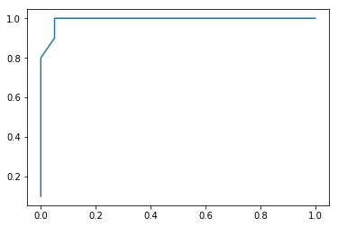
This is a good model!
Brier Score
The Brier score is the same as the mean squared error but is used on models that output probabilities. \(\sum _{i=1}^N (y^{(i)} - \hat y^{(i)})^2\)
Calibration Curve
The calibration curve is a graph where the x-axis has ranges of predictions and the y-axis has the proportion of positive samples for each range. This shows how well calibrated your model is by plotting predictions against actual positives.
A straight line with gradient of 1 is an ideal ‘well calibrated’ model.
Estimating Expected Loss
Train/Test Split
As test set size $\to \infty$ then the test error will converge to the true error (law of large numbers)
Cross Validation
Cross validation involves splitting a dataset into three subsets;
- Training set - Train model
- Validation set - Choose hyperparameters
- Test set - Estimate risk
K-Fold Cross-Validation
The training set is split into K chunks, iteratively trained on K-1 sets and tested on the Kth set to reduce overfitting. This helps to estimate the generalization error which is the risk of the function. It is also useful for evaluating how many features to include in the training set to minimize both approximation and estimation error. When K=N this is called ‘leave-one-out’ cross validation.
- Divide data into K partitions of roughly equal size (typically K is 4-10)
- For i in K:
- Train model using the dataset excluding fold K ($D_{-K}$)
- Test model on the kth fold of dataset ($D_K$)
- The output is a sequence of error measures. We should take the mean and standard deviation of the errors
Example:
Iteration 1: test = $D_1$, train = $D_2, D_3, D_4, … D_K$
Iteration 2: test = $D_2$, train = $D_1, D_3, D_4, … D_K$
Iteration K: test = $D_K$, train = $D_1, D_2, D_3, … D_{K-1}$
Stratified Sampling
This method is used to ensure representative test and train groups. It involves dividing the dataset into homogenous subgroups and sample the training set from each subgroup. Combining this with K-Fold cross validation is called Stratified K-Fold
Example:
11111100 -> train:[1110], test=[1110]