Stats #2: Distributions
Probability Distribution Functions
Probability distribution functions are used to map probabilities over a range.
Probability Mass Function (PMF)
A function that describes a dicrete distribution is called a probability mass function. The probability mass function of a discrete random variable is the probability it is exactly equal to some value $x$.
\[f_X(x) = P(X=x)\]Example: (2-coin toss)
If X = # of heads
$F_X(0) = 0.25$
$F_X(1) = 0.5$
$F_X(2) = 0.25$
Cumulative Distribution Function (CDF)
This describes the probability of $X$ being less than or equal to some value $x$. It is called cumulative as the probability will always increase as the value of $x$ increases.
\[F_X(x) = P(X \leq x)\]Example: In the coin toss example this function would represent the probability that the number of heads $X$ being less than or equal to 0, 1, or 2 respectively.
$x$ (No. of heads) $F_X(x)$ (Prob of $\leq$ x) Cases 0 0.25 TT 1 0.75 HT, TH, TT 2 1 HH, HT, TH, TT
Probability Density Function (PDF)
A function that describes a continuous distribution is called a probability density function.
The PDF of a continuous random variable is the relative likelyhood (NOT probability) of the variable lying between two points a & b. The probability is found by taking the area under the PDF curve by integration.
\[\int_a^bf_X(x)dx = P(a \leq X \leq b)\]Example
X is a uniform random variable [0-1]
\(P(0 \leq X \leq 0.3) = \int_0^{0.3}f_X(x)dx = 0.3\)
Random Distribution Functions
‘Random’ variables are rarely actually random, they usually conform to some type of distribution.
Types of Random Distribution
- Continuity (possible intervals for values)
- Discrete
- Continuous
- Variance (number of random variables)
- Univariate
- Bivariate
- Multivariate
- Support (possible number of outcomes)
- Finite
- Infinite
Some of the most common random distributions are listed below.
| Name | Type | Parameters | Description |
|---|---|---|---|
| Normal / Gaussian | Continuous | Mean ($\mu$), stdev ($\sigma$) | The ‘bell curve’ - most numbers cluster at average with fewer at either extreme |
| Exponential | Continuous | $e$ | Gradient increases as x increases |
| Poisson | Discrete | $\mu$ | Describes the number of events likely to occur in a time period based on the mean, $\mu$ |
| Binomial | Discrete | $n$, $P$ | Models $n$ successive independent binary trials each with $P$ probability of success |
| Bernoulli | Discrete | $P$ | Distribution of a process that has two possible outcomes where the positive has a probability of P |
| Geometric | Discrete | $P$ | A negative case of the binomial that is based on the number of trials required for 1 success |
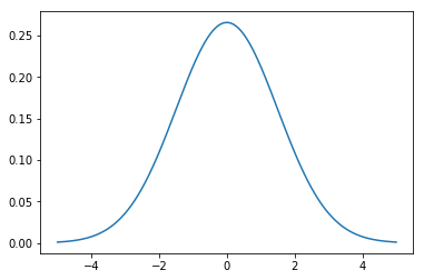
Gaussian
Also known as the normal distribution it is a very general case, and can be applied to almost every situation by the virtue of Central Limit Theorem. The shape is known as a bell curve and it is symmetric about the mean.
Plotting the Normal PDF in Python:
import scipy.stats as ss
import matplotlib.pyplot as plt
import numpy as np

fig, ax = plt.subplots()
x = np.linspace(-5, 5, 1000)
ax.plot(x, ss.norm.pdf(x, 0, 1.5))
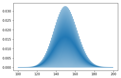
Poisson
A random variable X denoting the number of times a rare event occurs follows a Poisson distribution as the number of trials become large. Poisson is positively skewed and tends to normal as its mean $\mu$ becomes sufficiently large.
Plotting Poisson PMF in Python with $\mu=100$:
fig, ax = plt.subplots(1, 1)
mu = 100
x = range(0, 10)
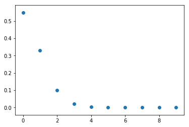
ax.scatter(x, poisson.pmf(x, mu))
With $\mu=0.6$:
Joint Probability Distributions
Given two random variables x and y:
DISCRETE (Joint PMF)
\[f_{XY}(x,y) = P(X=x, Y=y)\]CONTINUOUS (Joint PDF)
\[\int_c^d\int_a^b f_{XY}(x,y) = P(X \in [a,b], y \in [c,d])\]Example:
X: # Heads on first toss
Y: # Heads on second toss
$f_{XY}(0,0)$: Probability of X & Y being 0
$\omega$ $X(\omega)$ $Y(\omega)$ HH 1 1 HT 1 0 TH 0 1 TT 0 0 $f_{XY}(0,0) = P(X=0,Y=0) = P({TT}) = 0.25$
Joint Distributions for Independent Random Variables
Given two independent random variables x and y:
\[f_{XY}(x,y) = f_X(x)f_Y(y)\]Conditional Distributions
Some distributions can only be defined for some condition of the data.
$f_{Y|X}$: PMF/PDF of Y given X
Example: The distribution of heights in the population is a normal distribution if applied gender-wise. $f_{height|gender}$: Normal Dist (given gender)