Stats #4: Functions
Spaces
X: Input Space (Typically $\mathbb R^P$ where $\mathbb R^P$ is a real valued vector of P dimensions and P = # of predictors)
y: Output Space (In regression typically $\mathbb R$)
A: Action Space (Predictions)
In regression y=A.
Loss functions
A loss function is used to penalize bad predictions. It is applied to the output and predicted output values $y$ & $\hat y$ respectively.
\[(y,\hat y) \rightarrow L(y,\hat y)\]Absolute error loss
Absolute error is used for more noisy data or if there are outliers
\[L(y,\hat y) = |y -\hat y|\]Squared error loss
\[L(y,\hat y) = (y -\hat y)^2\]Margin based
\[L(y,\hat y) = f(y\hat y)\]Hinge loss
Used mostly for Support Vector Machines (SVM’s)
\[L(y,\hat y) = max(1-y\hat y, 0)\]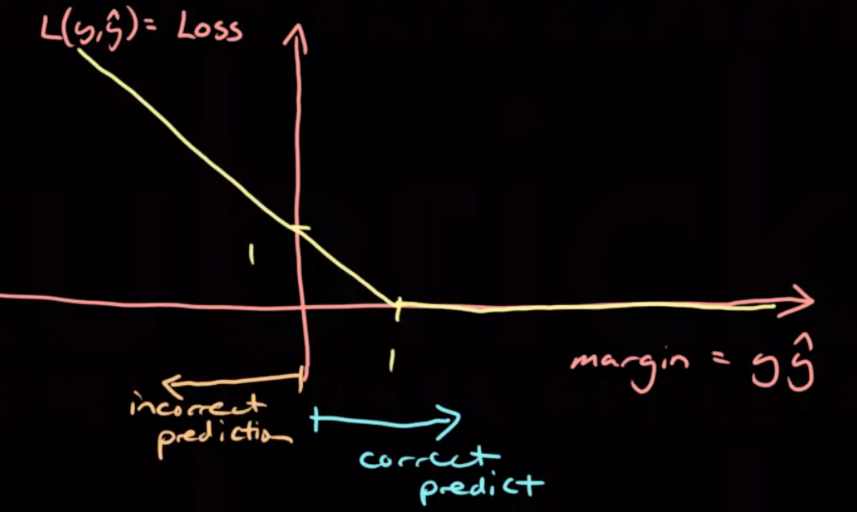
Misclassification Loss
For classification problems
\[L(y,\hat y) = 1(y \neq \hat y)\]0 if $y = \hat y$,
1 if $y \neq \hat y$
Log loss:
\[L(y,\hat y) = ylog(\hat y) - (1-y)log(1-\hat y)\]Where $y \in {0,1}$ & $\hat y \in [0,1]$
Risk
Risk Functional
The risk functional gives the expected loss when using f as the prediction function.
\[R(f) = E[L(y,f(X))]\]Empirical Risk Functional
This is essentially the average loss of the training points.
\[\hat R(f) = \frac1N \sum_{i=1}^N L(y^{(i)}, f(x^{(i)}))\]When empirical risk is wrong:
- If the distribution function is based on the training data then it will be flawed, then the calculated loss will be wrong. For this reason we must always split the input data into seperated training and testing sets and only use test data to estimate expected loss.
- If the space of functions is too large
- If the input data does not have ‘spreading information’; similar points at input should have similar predictions
Empirical Risk Minimizer
This is a function that best minimizes the empirical risk.
\[\hat f = argmin_f \hat R(f)\]Constrained Risk Minimizer
If $\mathscr F$ is a space of prediction functions the CRM attempts to minimize risk by changing the function space:
\[f_{\mathscr F}^* = argmin_{f \in \mathscr F} R(f)\]Constrained Empirical Risk Minimizer:
\[\hat f_{\mathscr F} = argmin_{f \in \mathscr F} \hat R(f)\]Excess Risk
The excess risk of a function is the function risk minus the bayes’ risk. It describes the risk that could be avoided. Excess risk can never be negative.
\[ER(f) = R(f) - R(f^*)\]Excess Risk Decomposition
If we consider the excess risk for the Constrained Empirical Risk Minimizer;
\[ER(\hat f_{\mathscr F}) = R(\hat f_{\mathscr F}) - R(f^*)\]The equation can be expanded to
\[ER(\hat f_{\mathscr F}) = R(\hat f_{\mathscr F}) - R(f_{\mathscr F}^*) + R(f_{\mathscr F}^*) - R(f^*)\](Where $R(f_{\mathscr F}^*)$ is the best risk within the constrained function space.)
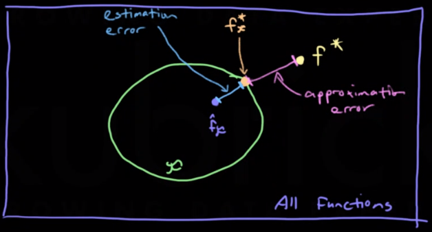
This expanded equation can be decomposed to form two seperate error measures.
Estimation Error / Variance:
The error between the function and the best function in the constrained space
Approximation Error / Bias:
The error between the best function in the constrained space and the bayes function
There is typically a trade off between estimation and approximation errors. We want a constrained function space $\mathscr F$ to reduce estimation error but the smaller the space is the larger the approximation error.
Approximation/Estimation Error Trade-off
High bias/approximation error = Underfitting (Model is independent of training data)
High variance/estimation error = Overfitting (Model is too dependent on training data)
If $\tau$ is a random fixed size training set, we can add an error variable $\epsilon$ to the prediction function $f(X) = E[y|X]$ to give $y=f(X) + \epsilon$. The error variable has an expectation $E[\epsilon] = 0$, and $(y_0, x_0)$ is a new fixed arbitrary point, the expected MSE can be expanded to show the different error types.
\[E_\tau[(y_0- \hat f(x_0))^2]\] \[= E_\tau[y_0^2- 2y_0 \hat f(x_0) + \hat f(x)^2]\] \[= E_\tau[(f(x_0) + \epsilon)^2 - 2(f(x_0) + \epsilon)\hat f(x_0) + \hat f(x_0)^2]\] \[= E_\tau[\epsilon^2] + E_\tau[f(x_0)^2 - 2f(x_0)\hat f(x_0) + \hat f(x_0)^2]\] \[= \sigma_\epsilon^2 + f(x_0)^2 - 2f(x_0)E_\tau[\hat f(x_0)] + E_\tau[\hat f(x_0)]^2 - E_\tau[\hat f(x_0)]^2 + E_\tau[\hat f(x_0)^2]\] \[= \sigma_\epsilon^2 + (f(x_0) - E[\hat f(x_0)])^2 + var(\hat f(x_0))\]- irreduceable error: $\sigma_\epsilon^2$
- Bias squared (approximation): $(f(x_0) - E[\hat f(x_0)])^2$
- Variance (estimation): $var(\hat f(x_0))$
Bayes Prediction Function
The Bayes’ prediction function (aka the target function) is the function that minimizes the expected loss, it the theoretical best function.
\[f^* = argmin_fR(f)\]$argmin_fR(f)$ returns the value for f that gives the lowest $R(f)$ value.
Bayes’ Prediction Function for a Squared Error Loss
Given $X=x_0$, if we wanted to predict $y$ with value $c$, we minimise the following expected loss:
\[E[(y-c)^2|X=x_0]\] \[= E[y^2-2cy+c^2|X=x_0]\]Take derivative:
\[\frac {\delta}{\delta c}E[y^2-2cy+c^2|X=x_0]\] \[= E[-2y + 2c|X=x_o]\]Set equal to zero (find minimum):
\[= -2E[y|X=x_0] + 2c = 0\] \[c = E[y|X=x_0]\]This means that Bayes’ prediction function for the square error loss is the conditional expectation.
\[f^*(x) = E[y|X=x]\]