Predicting Flood Risk for the UK
For 2 weeks in April 2019 I was part of a team tasked with creating a flooding risk prediction model and interface that could be used by an insurer to view risk by postcode across the UK.
Introduction
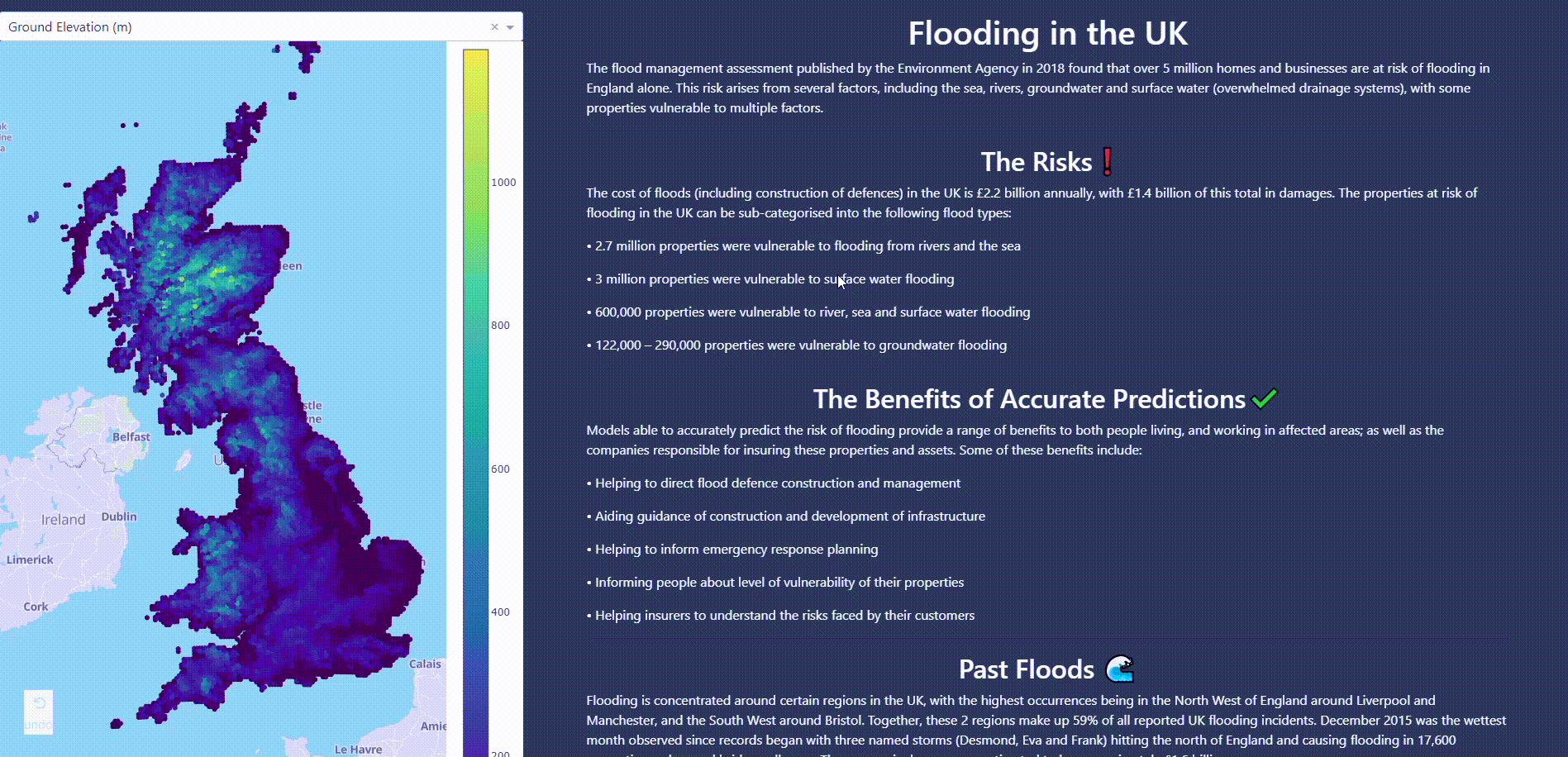
The flood management assessment published by the Environment Agency in 2018 found that over 5 million homes and businesses are at risk of flooding in England alone. Knowing where and when a dangerous flood could happen is vitally important to residents and businesses, as well as their insurers.
Our plan was first to source and clean reliable datasets of parameters such as weather, topography, proximity to water sources, historic floods and flood defences that could be included in our data warehouse.
Next we would train a predictive classification model which calculates a flood risk value between 0 and 1 for any UK Postcode.
The output of our model would be fet to a front end dashboard with interactive maps and charts showing both the input parameters and predicted risk for a selected UK postcode.
I will introduce the data sources, show some of the code, and the final dashboard in the order described.
Data
Primary datasets
The primary table we used was a 5km x 5km grid of the UK, each with a grid reference and a geographicly described polygon. Ordnance Survey grids are available on Github for multiple grid sizes in both GeoJSON and Shapefile format.
The other key base dataset we required was postcodes and their respective polygons. While the model would be trained at the grid level we would then aggregate the results to a postcode granularity in order for the tool to be able to be indexed by postcode. Geolytix has a useful postcode database that we used.
Weather data
Rainfall and wind data was sourced from The Centre for Environmental Data Analysis.
Rainfall, river flow and river catchment boundary data is available from the Centre for Ecology and Hydrology National River Flow Archive.
For our model we used rainfall, wind and temperature data. The weather data were downloaded in txt format, and the weather station location data were downloaded in xls format, both were distributed across many files. The data were converted to csv format and imported to Python. The data were concatenated into four data tables: rainfall, wind, temperature and station data. These tables were then exported to SQL, where they were cleaned. Weather features were created by aggregating over station IDs, years and quarters.
The station location table which contained point geometry was used to link the three weather tables back to the original 5km grid. If a gridbox contained a station point, the station was assigned to the gridbox. If a gridbox contained several station points, the station with the most recent time stamp was chosen. If a gridbox didnt contain a station, information from the nearest station was used.
Terrain
Granular elevation data for the whole of the UK is available from the Ordnance Survey. River geographic lines are also available from the Ordnance Survey. Data on UK flood defences is published by the Environment Agency
The elevation data were distributed between two data sets: elevation by postcode referenced by central point and elevation at ordinance survey points throughout the UK. Both were downloaded in csv format, imported to SQL and unioned into one dataset with point geography. These data were then matched with the 5km grid to create three features:
- Mean elevation within each gridbox
- Standard deviation of elevation within each gridbox
- The difference between the mean elevation of a gridbox and the average of the mean elevations of all neighbouring gridboxes. This indicated whether the gridbox was more or less elevated than its neighbours.
Historical Flooding
There are a number of data sources for flooding data such as data.gov. The modelling team collated these into a prediction column ‘y’ of flooding risk.
A source of floods in the past 1 year, 3 years, 6 years and 11 years was used. The flooding areas were intersected with the 5km grid to produce a table of flooding history for each grid square. The table was then cleaned and split into the train and test data with 80:20 ratio.
The training data had few instances of locations that did flood compared to the number of locations that never flooded. This imbalance can lead to the model not correctly identifying flooding instances. Bootstrapping was used to sample different ratios of flooding to not-flooding with a final upsampling rate selected was 37.5% flooded to 62.5% not flooded.
Model
We decided to use a random forest classification model as they are known to be effective using many input variables of both categorical and continuous type. It also allows for easy examination of varible importance, enabling us to efficiently select the most influential variables. The model outputs a probability between 0 and 1 indicating how likely that gridbox is to flood over the selected timeframe (1 year, 3 years, 6 years or 11 years).
Model Construction
The model was constructed exclusively in Python, using the following modules and packages:
- matplotlib.pyplot
- pyodbc
- pandas
- random.randrange
- numpy
- sklearn.ensemble.RandomForestClassifier
- sklearn.metrics
- sklearn.metrics.classification_report
- sklearn.model_selection.GridSearchCV
- seaborn
The model was tuned by changing the values of the following hyperparameters:
- Number of estimators
- Maximum tree depth
- Number of feaures to consider at each split
- Type of split
The optimum hyperparameters were decided by analysing the precision, recall and f1 score analysis. The recall score was prioritised over precision, as the intended customer is an insurance company for whom a correctly predicted flood is more important than a correctly predicted non flood. To select the optimal hyperparameters we used the recall value multiplied by the f1 score.
Our tests showed that the 6 year model with the hyperparameters: criterion = entropy, maximum depth of the tree = 13, maximum number of features considered at each split = \sqrt{n}, number of estimators = 750 yielded the best results, so this was selected as the final model. Given more time the modelling team would have trialled neural networks and XGBoost for possible improvements.
We combined the output column of the model with the original fact table for the 5km grid. The postcode sector was then assigned to every gridbox by taking the central point of the gridbox polygons and finding which sector it was located in. The data in the table were then aggregated by sector, and cleaned by backfilling null values. We classified the flood risk into ten sections, and asigned a specific colour to each one. To increase computational efficiency geometry values were rounded to 3 decimal places which significantly reduced the size of the final table. This table was then converted to Geojson format. An analogous table was created for postcode areas.
Dashboard
To visualise the model outputs we decided to create an interactive Web-based application using Dash. The webpage is split into three tabs: Background, Tools and Derivation. All three tabs are interactive with user input in the Tools tab.
Background
The first page of the final product explains some background on flood risk and hosts a map showing a chosen feature of the dataset.
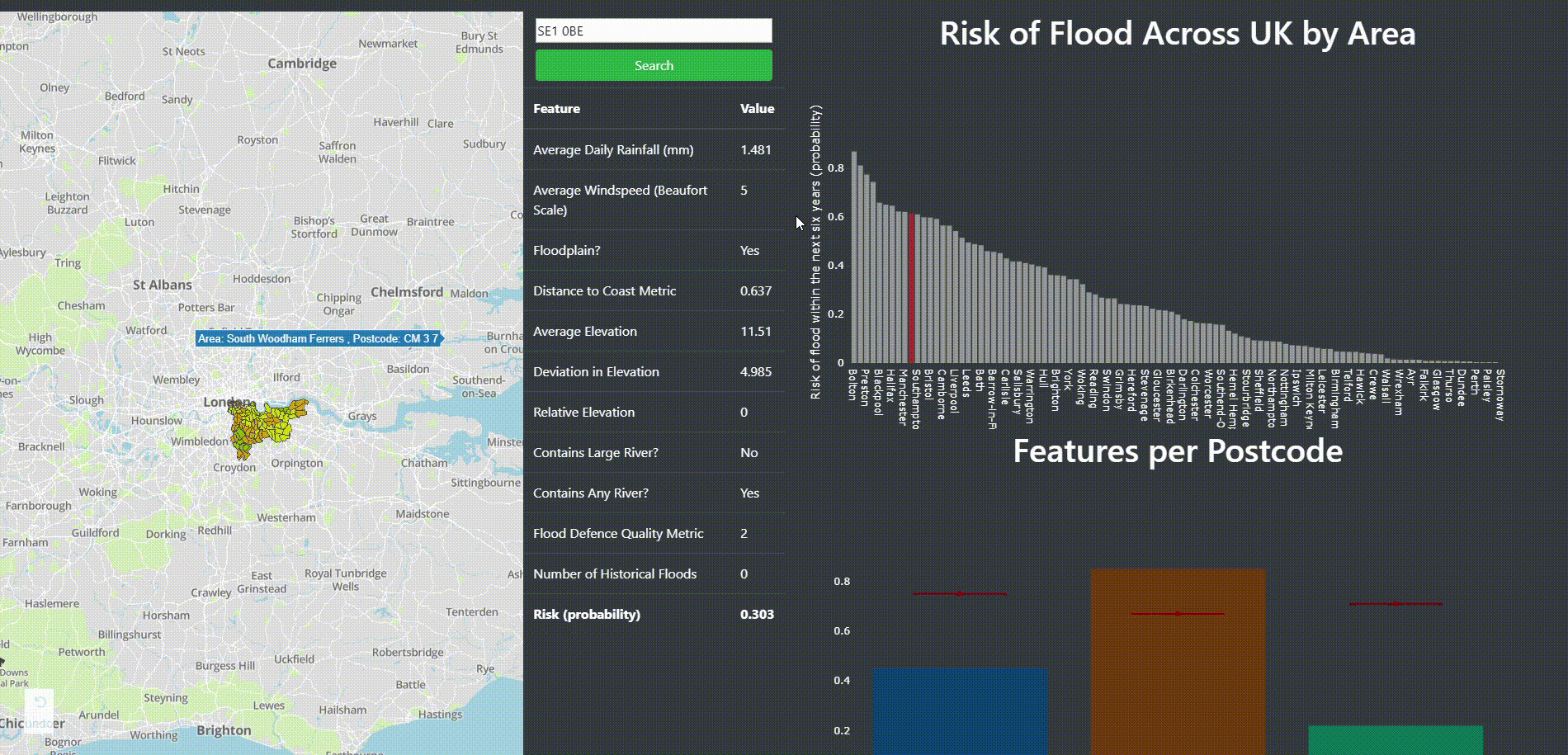
Tool
The main tool has a search box that accepts post code entries, once entered the map will move to the selected postcode area and show flood risk by postcode sector using a colour scale. Below the search bar the key input features are shown as well as the aggregated model output; the risk for a sector. The top right graph shows how the risk of that postcode area compares to the rest of the country. The bottom right graph shows scaled values of rainfall, distance from coast, and elevation of the sector as well as the averages.
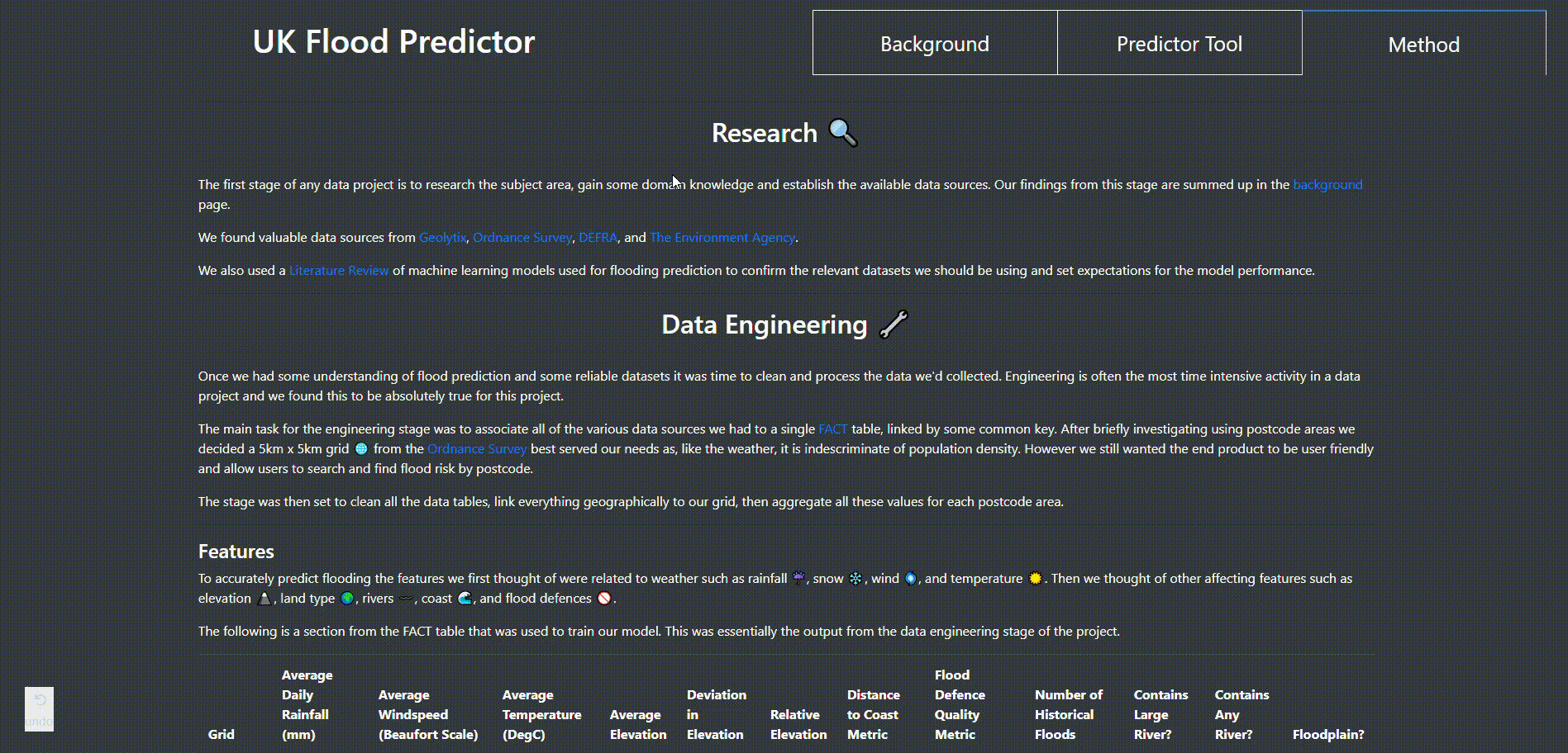
Method
The last page explains the method that was taken during the project including research, engineering, model training, & visualisation. It also has a subset of the feature table and a tool to graph different features against eachother to check for any dependencies.